Finding and Fixing Autocorrelation

The HRF derivative effects shown on the second row represent the change in average ACI when including the HRF derivative in each GLM [βk(v) in model 2]. The mean effect shows that including HRF derivatives tends to decrease ACI, particularly in areas where ACI tends to be the highest, as observed in Figure 1. The task-specific deviations show that more flexible HRF modeling has the strongest effect for the motor task, mimicking the more severe autocorrelation seen in the motor task. The areas most affected by flexible HRF modeling for each task tend to somewhat mimic the spatial patterns unique to each task, but do not fully account for them. These include carryover effect, where effects from a prior test or event affect results.

Sometimes the variance of the error terms depends on the explanatory variable in the model. It is necessary to test for autocorrelation when analyzing a set of historical data. For example, in the equity market, the stock prices on one day can be highly correlated to the prices on another day.

Autocorrelation Introduction

Although a very useful tool, it is often used with other statistical measures in financial analysis. For example, in time-series regression involving quarterly data, such data are usually derived from the monthly data by simply adding three monthly observations and dividing the sum by 3. This averaging introduces smoothness into the data by dampening the fluctuations on the monthly data.

• The following section evaluates the effect of different prewhitening strategies on mitigating autocorrelation, reducing spatial variability in autocorrelation, and controlling false positives.
• A valuable topic of future work would be to develop prewhitening methods that formally model and adjust for this source of bias.
• Dotted lines correspond to accounting for the degrees of freedom (DOF) lost when estimating AR coefficients.
• In many circumstances, autocorrelation can€™t be avoided; This is especially true of many natural processes including some behavior of animals, bacteria [2], and viruses [1].

Current prewhitening methods implemented in major fMRI software tools often use a global prewhitening approach. One likely reason for this is the computational efficiency of global prewhitening, since it requires a single T×T matrix inversion, unlike local prewhitening which requires V such inversions. Likewise, the GLM coefficients can be estimated in a single matrix multiplication step with global prewhitening, whereas local prewhitening requires V multiplications.

(A) The optimal AR model order at every vertex for a single subject for each task. The optimal order clearly varies across the cortex and with the task being performed. (B) The distribution of optimal AR model order across all vertices, averaged over all subjects, sessions and tasks.

There are many features of task fMRI data that may not be reflected in resting-state fMRI data. For example, mismodeling of the task-induced HRF can induce residual autocorrelation, as shown in Figure 1. Inclusion of HRF derivatives only partly accounts for the task-related differences in autocorrelation, as shown in Figure 2. Second, we quantify false positives using resting-state fMRI data, assuming a false boxcar task paradigm.

Extract SQL tables, insert, update, and delete rows in SQL databases through SQLAlchemy

The optimal AR model order is two or less for most vertices, but over 20% of vertices have optimal AR model order of 3–6, while over 10% have optimal order of 7 or higher. Population variability in the effects shown in Figure 2, based on the random effect (RE) standard deviations (SD) from model (2). The first column shows the average across tasks, indicating general spatial patterns of population variability. The other columns show the difference between each task and the average, indicating areas of greater (warm colors) or lesser (cool colors) variability during specific tasks. The first row shows variability in autocorrelation when assuming a canonical HRF [ak, i(v)]; the second row shows variability in the effect of using HRF derivatives to allow for differences in HRF shape [bk, i(v)]. The sum of both effects shown in the third row represent the average ACI when including HRF derivatives [αk(v)+βk(v) in model 2].

We generate autocorrelated timeseries for each voxel using an AR(3) model with white noise variance equal to 1. The AR coefficients are chosen to induce low ACI in white matter, moderate ACI in gray matter, high ACI in CSF, and unit ACI (the minimum) in background voxels. Finally, one limitation of our implementation of AR-based prewhitening implementation is that we did not account for potential bias in the prewhitening matrix due to using the fitted residuals as a proxy for the true residuals. Since the fitted residuals have a different dependence structure induced by the GLM, their covariance matrix is not equal to that of the true residuals. This bias will generally be worse in overparameterized GLMs, which may help explain why we observed a slightly detrimental effect of including all 24 motion regressors when prewhitening was also performed (see Figure A.1 in Appendix). A valuable topic of future work would be to develop prewhitening methods that formally model and adjust for this source of bias.

3. Low-order AR models perform surprisingly well when allowed to vary spatially

Those distortions cause a slight misalignment of the fMRI data on the structure of the brain. This has the result of mixing CSF signals with higher autocorrelation into some cortical areas, and mixing white matter signals with lower autocorrelation into others. As a result, in the HCP there may be sizeable discrepancies in false positive control and power across and within each hemispheres before prewhitening or when using global prewhitening. Different acquisitions may therefore produce very different spatial distributions of false positive control, if not addressed through an effective local prewhitening strategy.

(C) Mean ACI over subjects and sessions, averaged across all vertices, by task and prewhitening method. Notably, allowing AR model coefficients to spatially vary reduces ACI much more than increasing AR model order. Our study, as well as most prior studies on the efficacy of prewhitening in task fMRI analyses, focused on the ability of prewhitening techniques to effectively mitigate autocorrelation and control false positives. Here we discussed, but did not explicitly analyze, the possibility of a loss of power due to over-whitening.

In this article, let’s dive deeper into what are Heteroskedasticity and Autocorrelation, what are the Consequences, and remedies to handle issues. The autocorrelation analysis only provides information about short-term trends and tells little about the fundamentals of a company. Therefore, it can only be applied to support the trades with short holding periods. Although autocorrelation should be avoided in order to apply further data analysis more accurately, it can still be useful in technical analysis, as it looks for a pattern from historical data. The autocorrelation analysis can be applied together with the momentum factor analysis. Autocorrelation can be applied to different numbers of time gaps, which is known as lag.

Similar to Autocorrelation- Concept, Causes and Consequences(

Rain runs a regression with the prior trading session’s return as the independent variable and the current return as the dependent variable. They find that returns one day prior have a positive autocorrelation of 0.8. Even if the autocorrelation is minuscule, there can still be a nonlinear relationship between a time series and a lagged version of itself. An autocorrelation of +1 represents a perfect positive correlation (an increase seen in one time series leads to a proportionate increase in the other time series). DP, DS, and AM developed the methods and software for the prewhitening techniques evaluated in the paper. FP and AM wrote the first draft of the manuscript, while RW and DP wrote sections.

In general, p-order autocorrelation occurs when residuals p units apart are correlated. When using Markov chain Monte Carlo (MCMC) algorithms in Bayesian analysis, often the goal is to sample from the posterior distribution. We resort to MCMC causes of autocorrelation when other independent sampling techniques are not possible (like rejection sampling). The problem however with MCMC is that the resulting samples are correlated. This is because each subsequent sample is drawn by using the current sample.

2. Implications for volumetric fMRI analyses

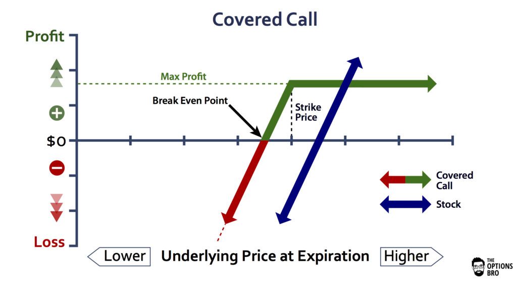
On the other hand, an autocorrelation of -1 represents a perfect negative correlation (an increase seen in one time series results in a proportionate decrease in the other time series). If the price of a stock with strong positive autocorrelation has been increasing for several days, the analyst can reasonably estimate the future price will continue to move upward in the recent future days. The analyst may buy and hold the stock for a short period of time to profit from the upward price movement. Autocorrelation refers to the degree of correlation of the same variables between two successive time intervals. It measures how the lagged version of the value of a variable is related to the original version of it in a time series.

The Durbin-Watson tests produces a test statistic that ranges from 0 to 4. Values close to 2 (the middle of the range) suggest less autocorrelation, and values closer to 0 or 4 indicate greater positive or negative autocorrelation respectively. However, autocorrelation can also occur in cross-sectional data when the observations are related in some other way. In a survey, for instance, one might expect people from nearby geographic locations to provide more similar answers to each other than people who are more geographically distant. Similarly, students from the same class might perform more similarly to each other than students from different classes. Thus, autocorrelation can occur if observations are dependent in aspects other than time.

We can see in this plot that at lag 0, the correlation is 1, as the data is correlated with itself. At a lag of 1, the correlation is shown as being around 0.5 (this is different to the correlation computed above, as the correlogram uses a slightly different formula). We can also see that we have negative correlations when the points are 3, 4, and 5 apart.

Effect of including additional motion covariates on autocorrelation, when effective prewhitening is performed. For prewhitening, we use an AR(6) model with local regularization of AR model coefficients, which we observe to be highly effective at reducing autocorrelation. The first two columns show the average autocorrelation index (ACI) across all subjects, sessions and tasks when 12 realignment parameters (RPs) or 24 RPs are included in each GLM.

Eight different prewhitening strategies are shown, based on four different AR model orders (1, 3, 6, and optimal at each vertex) and two different regularization strategies for AR model coefficients (local smoothing vs. global averaging). Higher AR model order and allowing AR model coefficients to vary spatially results in substantially greater reduction in the number of vertices with statistically significant autocorrelation. Notably, allowing AR model coefficients to spatially vary has a greater effect than increasing AR model order. (C) Percentage of vertices with statistically significant autocorrelation, averaged across all subjects, sessions, and tasks. Dotted lines correspond to accounting for the degrees of freedom (DOF) lost when estimating AR coefficients.